Optimization models in Python with PuLP

November 7, 2026 · 7 min read

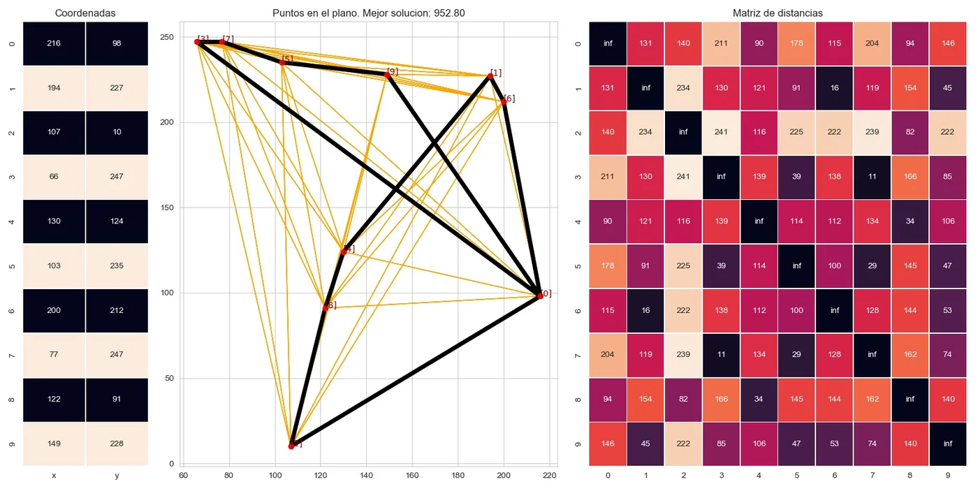
This post is a written version of an invited lecture on Python for optimization and logistics that I taught at the Universidad San Francisco Xavier de Chuquisaca (USFX), in Sucre, Bolivia. The lectures follows four classic problems: placing two hospitals, the p-median problem, the traveling salesman problem and vehicle routing.

Tools

The models use PuLP, a Python library for writing linear programs, which calls GLPK (an open-source mixed integer linear programming solver) behind the scenes.

python -m pip install pulp

PuLP also ships with the CBC solver. If GLPK is not installed, replace GLPK(options=['--mipgap', '0.01']) in the code below with PULP_CBC_CMD(gapRel=0.01). Both stop once the solution is within 1% of the optimum.

A small helper file, utils.py, creates the variables in bulk and runs the solver:

from pulp import *

def create_variable_matrix(i, j, name="x_{i}_{j}", **other_args):
    return [[LpVariable(name.format(i=a, j=b), **other_args) for b in range(j)]
            for a in range(i)]

def create_variable_array(i, name="y_{i}", **other_args):
    return [LpVariable(name.format(i=a), **other_args) for a in range(i)]

def euclidian_distance(point1, point2):
    return ((point1[0] - point2[0]) ** 2 + (point1[1] - point2[1]) ** 2) ** 0.5

def create_distance_matrix(points):
    return [[euclidian_distance(a, b) for b in points] for a in points]

def resolve_problem(problem, show_variables=True):
    GLPK(options=['--mipgap', '0.01']).solve(problem)
    if show_variables:
        for v in problem.variables():
            if v.varValue != 0:
                print(v.name, "=", v.varValue)
    return value(problem.objective)

Note that LpVariable takes three main params: cat, the kind of variable ('Continuous' or 'Integer'); lowBound, its minimum (\(-\infty\) when omitted); and upBound, its maximum (\(+\infty\) when omitted).

An integer variable between 0 and 1 is a yes-or-no decision. A \(5 \times 10\) matrix of them, and a list of 17 non-negative integers can be written as:

f = create_variable_matrix(5, 10, name="F_{i}_{j}", cat='Integer', lowBound=0, upBound=1)
l = create_variable_array(17, name="L_{i}", cat='Integer', lowBound=0)

A model has the class LpProblem. It has overloaded the operator += to allow an interesting syntax for adding constraint: model += constraint:

problem = LpProblem("my_model", LpMinimize)   # or LpMaximize

Model A: two hospitals

Seven neighborhoods need two new hospitals, each built in one of the neighborhoods. Where should they go?

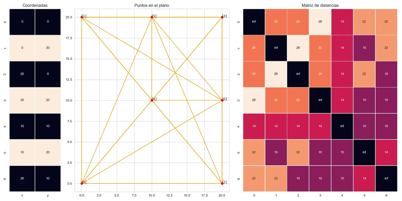
Three panels: a table of the coordinates of the seven neighborhoods, the neighborhoods as points in the plane joined by every possible connection, and a heat map of the distances between them. — The seven neighborhoods, every possible connection between them, and their distance matrix.

A good solution should keep every neighborhood close to the hospital that serves it, so the objective is the sum of the distances from each neighborhood to its hospital. That needs two kinds of decisions to be modeled:

\(x_{ij} = 1\) if neighborhood \(i\) is served by a hospital in neighborhood \(j\), and \(0\) otherwise, for \(0 \le i, j \le 6\).
\(y_j = 1\) if a hospital is built in neighborhood \(j\), and \(0\) otherwise.

problem = LpProblem("two_hospital_problem", LpMinimize)
x = create_variable_matrix(7, 7, cat='Integer', lowBound=0, upBound=1)
y = create_variable_array(7, name="y_{i}", cat='Integer', lowBound=0, upBound=1)

Where \(d_{ij}\) is the distance between neighborhoods \(i\) and \(j\), the objective is

\[\min \sum_{i=0}^{6} \sum_{j=0}^{6} d_{ij}\, x_{ij} = 0.0\,x_{0,0} + 20.0\,x_{0,1} + 20.0\,x_{0,2} + 28.3\,x_{0,3} + \dots + 14.1\,x_{6,5} + 0.0\,x_{6,6}.\]

This means that the objective function needs to link all possible \(7 * 7\) combinations:

objective = (0.0 * x[0][0] + 20.0 * x[0][1] + 20.0 * x[0][2] + 28.3 * x[0][3]
             + 14.1 * x[0][4] + 22.4 * x[0][5] + 22.4 * x[0][6]
             + 20.0 * x[1][0] + ...)                 # 49 terms in all
problem += objective

There is a trivial solution: \(x=0\), i.e., the solution that minimizes the distance between hospitals and neighborhoods is to not build any hospital at all. So, we need additional constraints to make a solution valid:

Every neighborhood is served by exactly one hospital: \(\sum_{j} x_{ij} = 1\) for every \(i\). For neighborhood 0 that is \(x_{0,0} + x_{0,1} + \dots + x_{0,6} = 1\), and the same holds for the other six.
There are exactly two hospitals: \(\sum_{j} y_j = 2\).
A neighborhood can only be served by a hospital that exists: if \(x_{ij} = 1\), then \(y_j\) must be 1. We can write this as a linear constraint, \(x_{ij} \le y_j\) for every \(i\) and \(j\).

for i in range(7):                              # 1. one hospital per neighborhood
    problem += lpSum(x[i][j] for j in range(7)) == 1
problem += lpSum(y) == 2                        # 2. two hospitals
for i in range(7):                              # 3. only hospitals that exist
    for j in range(7):
        problem += x[i][j] <= y[j]

resolve_problem(problem, show_variables=True)

If we run the code, GLPK prints its progress, then the variables that are not zero:

x_0_4 = 1
x_1_5 = 1
x_2_4 = 1
x_3_5 = 1
x_4_4 = 1
x_5_5 = 1
x_6_4 = 1

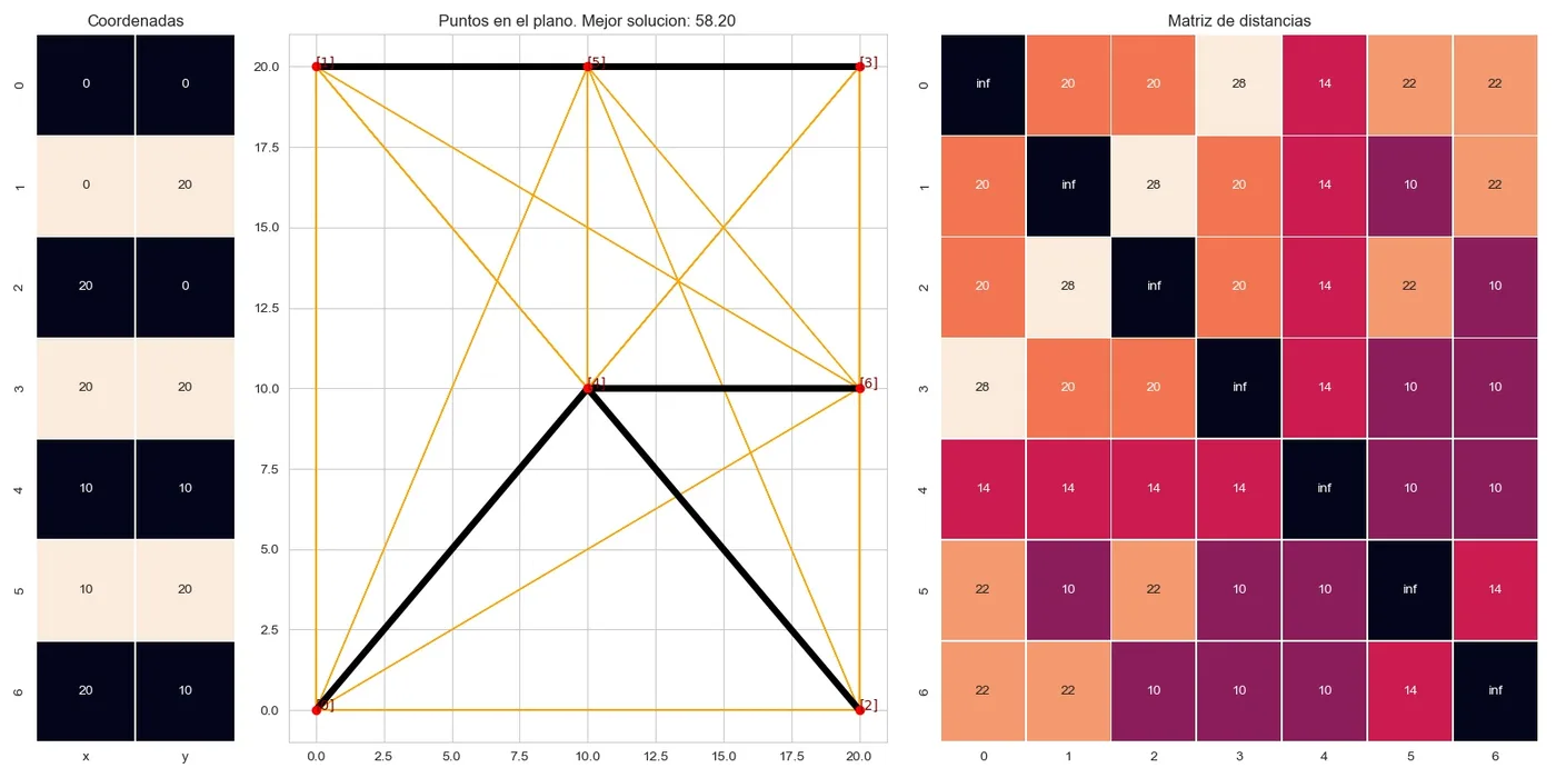
We can interpret this as the hospitals should be built in neighborhoods 4 and 5. Neighbourhoods 0, 2, 4 and 6 use the hospital in 4; neighborhoods 1, 3 and 5 use the one in 5. The total distance is 58.2.

Solution drawn in black: two star-shaped groups of connections, centered on neighborhoods 4 and 5

Model B: p-median problem

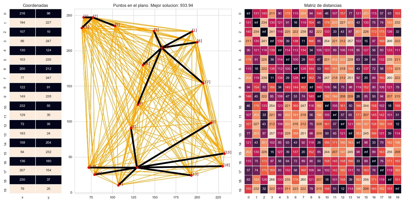
The two-hospital model is a special case of a location problem. There are \(n\) customers to serve and \(m\) places where a service point could open. The p-median problem opens \(p\) of them and assigns every customer to one open service point, so that the sum of the distances from the customers to their service points is as small as possible.

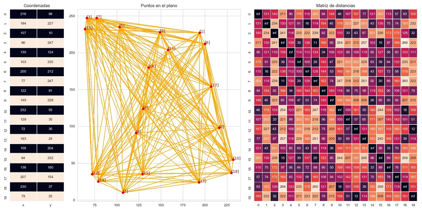
20 random points joined by every possible connection

The variables are similar to those in model A: \(y_j = 1\) if a service point opens at \(j\), and \(x_{ij} = 1\) if customer \(i\) is served from \(j\). So is the model, with \(p\) in place of 2:

\[\begin{aligned} \min\ & \sum_{i=1}^{n} \sum_{j=1}^{m} d_{ij}\, x_{ij} \\ \text{subject to}\ & \sum_{j=1}^{m} x_{ij} = 1, && i = 1, \dots, n, \\ & \sum_{j=1}^{m} y_j = p, \\ & x_{ij} \le y_j, && i = 1, \dots, n,\ j = 1, \dots, m, \\ & x_{ij}, y_j \in \{0, 1\} \end{aligned}\]

This time we can write this objective function can be written as loop for any number of points and any \(p\). To keep the example simple, every customer is also a candidate place (\(m = n\)):

def p_median_problem(distance_matrix, facilities):
    n = len(distance_matrix)
    problem = LpProblem("p_median_problem", LpMinimize)
    x = create_variable_matrix(n, n, cat='Integer', lowBound=0, upBound=1)
    y = create_variable_array(n, name="y_{i}", cat='Integer', lowBound=0, upBound=1)

    problem += lpSum(distance_matrix[i][j] * x[i][j] for i in range(n) for j in range(n))
    for i in range(n):                          # each customer served once
        problem += lpSum(x[i][j] for j in range(n)) == 1
    problem += lpSum(y) == facilities           # exactly p service points
    for i in range(n):                          # only from open service points
        for j in range(n):
            problem += x[i][j] <= y[j]

    return resolve_problem(problem)

The best three service points for the 20 customers

Model C: the traveling salesman

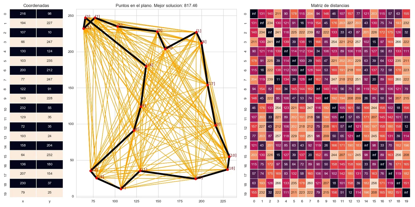
This is one of the most classical examples in linear programming or optimization. Assume we know \(n\) cities and the distances between them, the traveling salesman problem looks for the shortest route that starts in one city, visits each of the others exactly once and comes back.

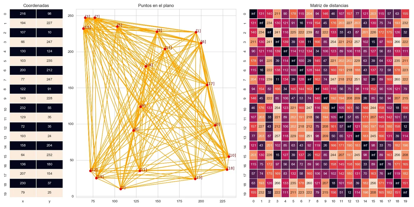
Let \(x_{ij} = 1\) if the route goes straight from city \(i\) to city \(j\), and \(0\) otherwise. Thus, the objective is the length of the route:

\[\min \sum_{i=1}^{n} \sum_{j=1}^{n} d_{ij}\, x_{ij}.\]

At first sight two constraints are enough and intutive enough: one road arrives at each city, and one road leaves it.

\[\sum_{i=1}^{n} x_{ik} = 1 \quad\text{and}\quad \sum_{j=1}^{n} x_{kj} = 1, \qquad k = 1, \dots, n.\]

for k in range(n):
    problem += lpSum(x[i][k] for i in range(n)) == 1   # one road in
    problem += lpSum(x[k][j] for j in range(n)) == 1   # one road out

Are those two enough? No!. This is a valid solution only using those two constraints:

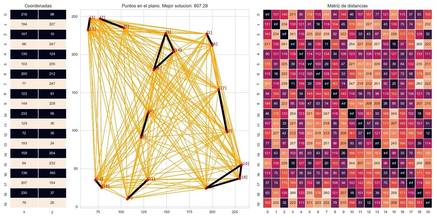
A solution using only 2 constraints may involve several small loops

The answer is correct for the model: every city has exactly one road in and one road out. Nothing in the model informs that the roads must form a single loop, and several short loops are cheaper than one long one. We often called these loops as subtours.

There are several ways to rule them out. We use the flow formulation (Gavish&Graves, 1978). They solve the subtours issue in a clever way: the idea was to add a new variable: \(f_{ij} \ge 0\), an amount of flow sent along the road from \(i\) to \(j\). This amount is not measured and does not appear in the objective function, but it works as a variable that appears while the model is running (like a temporary variable in a programming language!). Using it, now we can model that city 1 need to send out \(n - 1\) units, and every other city keeps exactly one:

\[\sum_{i=1}^{n} f_{ik} - \sum_{j=1}^{n} f_{kj} = 1, \qquad k = 2, \dots, n.\]

Flow can only travel along roads that the route uses, and since no road ever needs to carry more than \(n - 1\) units,

\[f_{ij} \le (n - 1)\, x_{ij}, \qquad i, j = 1, \dots, n,\ i \ne j.\]

A subtour that does not pass through city 1 has no road bringing flow in from outside, and each of its cities must keep one unit. That is impossible, so every city has to be on the same loop as city 1. For the same reason, a city cannot be its own loop (\(x_{kk} = 1\)), which is why the code does not have to exclude those variables.

def travelling_salesman_problem(distance_matrix):
    n = len(distance_matrix)
    problem = LpProblem("travelling_salesman_problem", LpMinimize)
    x = create_variable_matrix(n, n, cat='Integer', lowBound=0, upBound=1)
    f = create_variable_matrix(n, n, name="f_{i}_{j}", cat='Integer', lowBound=0)

    problem += lpSum(distance_matrix[i][j] * x[i][j] for i in range(n) for j in range(n))
    for k in range(n):
        problem += lpSum(x[i][k] for i in range(n)) == 1          # one road in
        problem += lpSum(x[k][j] for j in range(n)) == 1          # one road out
    for k in range(1, n):                                          # each city keeps one unit
        problem += lpSum(f[i][k] for i in range(n)) - lpSum(f[k][j] for j in range(n)) == 1
    for i in range(n):                                             # flow only on used roads
        for j in range(n):
            if i != j:
                problem += f[i][j] <= (n - 1) * x[i][j]

    GLPK(options=['--mipgap', '0.01', '--tmlim', '30']).solve(problem)
    return value(problem.objective)

The --tmlim 30 option stops GLPK after 30 seconds, so on larger instances the result is the best route found in that time, not necessarily the shortest one.

With the flow constraints, the solution is a single route through every city

Model D: vehicle routing

The vehicle routing problem could be seen as a expansion of the TSP, where we have more than one salesman (or trucks in this case) and the traveler can only bring a limited amount of supply or goods. A depot, point 0, serves \(n\) customers, numbered 1 to \(n\). Customer \(k\) needs \(q_k\) units of goods, and the depot needs none (\(q_0 = 0\)). There are as many vehicles as needed, each carrying at most \(Q\) units. The goal is the cheapest set of routes such that:

every route starts and ends at the depot,
every customer’s demand is delivered, and
no route carries more than \(Q\) units in total.

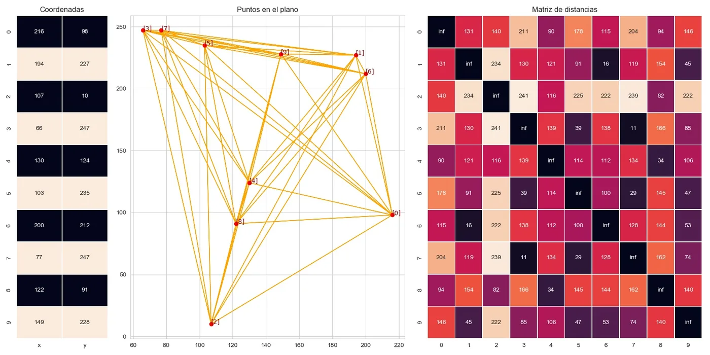
Defining \(c_{ij}\) as the cost of traveling from \(i\) to \(j\), the variables \(x_{ij} = 1\) if a vehicle goes from \(i\) to \(j\), and \(f_{ij} \ge 0\), the amount of goods carried from \(i\) to \(j\), the model is then:

\[\begin{aligned} \min\ & \sum_{i=0}^{n} \sum_{j=0}^{n} c_{ij}\, x_{ij} \\ \text{subject to}\ & \sum_{j=0}^{n} x_{kj} = 1, \quad \sum_{i=0}^{n} x_{ik} = 1, && k = 1, \dots, n, \\ & \sum_{j=1}^{n} x_{0j} = \sum_{i=1}^{n} x_{i0}, \\ & \sum_{i=0}^{n} f_{ik} - \sum_{j=0}^{n} f_{kj} = q_k, && k = 1, \dots, n, \\ & f_{ij} \le Q\, x_{ij}, && i, j = 0, \dots, n,\ i \ne j. \end{aligned}\]

Line by line the model can be interpreted as we did before:

One vehicle leaves and one arrives at each customer
As many vehicles come back to the depot as leave it
Each customer keeps exactly its demand from the goods that pass through it
And, no road carries more than a vehicle holds

The flow constraints play the same role as in the TSP model: goods can only start at the depot, so every route must pass through it.

def vehicle_routing_problem(distance_matrix, demand, vehicle_capacity):
    n = len(distance_matrix)
    problem = LpProblem("vehicle_routing_problem", LpMinimize)
    x = create_variable_matrix(n, n, cat='Integer', lowBound=0, upBound=1)
    f = create_variable_matrix(n, n, name="f_{i}_{j}", cat='Integer', lowBound=0)

    problem += lpSum(distance_matrix[i][j] * x[i][j] for i in range(n) for j in range(n))
    for k in range(1, n):
        problem += lpSum(x[k][j] for j in range(n)) == 1          # one vehicle leaves
        problem += lpSum(x[i][k] for i in range(n)) == 1          # one vehicle arrives
    problem += (lpSum(x[0][j] for j in range(1, n))                # depot: as many out as in
                == lpSum(x[i][0] for i in range(1, n)))
    for k in range(1, n):                                          # each customer keeps q_k
        problem += lpSum(f[i][k] for i in range(n)) - lpSum(f[k][j] for j in range(n)) == demand[k]
    for i in range(n):                                             # vehicle capacity
        for j in range(n):
            if i != j:
                problem += f[i][j] <= vehicle_capacity * x[i][j]

    return resolve_problem(problem)

In the example every customer needs one unit and a vehicle carries five, so the nine customers need at least two vehicles. The best plan uses exactly two, which could make their deliveries at the same time.

Optimal route: 2 vehicles with their own loop from the depot