Numerical Hell: When Cross-Language Code Breaks (Part 1)
I believe engineers have an unspoken rule: we trust our tools. When you design an IIR filter or an FIR filter, you expect identical results regardless of your programming language. While I suspected this assumption wouldn’t always hold, I never gave it much thought until recently.
Working with electrical brain signals, my lab analyzes bursts that could help identify seizure-generating tissue. Some of our legacy code runs in MATLAB, but I had my statistical and machine learning pipelines in Python. After having horrible experiences in the past with bugs while connecting MATLAB-Python, I had two options: either use an Python-Octave bridge (oct2py) or rewrite the algorithm in Python. Due to memory efficiency, I decided to port the algorithm entirely.
The plan was simple: implement everything identically and use a unit test battery that can confirm the results are the same. The code looked perfect until I ran the tests. To my surprise, around 20% failed. Well, it is known that some operations can raise sligtly different results on both platforms, as the inverse random transformation. Sometimes, due to the way the algorithm is implemented between MATLAB versions.
After two frustrating days of debugging, I isolated several issues. Let’s start with the simplest and most frustrating one: the FIR filter design functions (fir1 in MATLAB/Octave, firwin in scipy).
Minimal example
Here’s what we obtained as a FIR bandpass filter between 0.2\(f_s\) and 0.4\(f_s\) with a Hamming window (\(f_s\) is the sampling frequency) in Octave, python and R:
% Octave 9.3.0 / signal 1.4.6
pkg load signal
fir1(2, [0.1, 0.2], "bandpass")
% ans =
%    0.06310305169   0.88754953849   0.06310305169

% Matlab 2024b
format longg
fir1(2, [0.1, 0.2], "bandpass")
%ans =
%   0.063016142388235   0.887704412005799   0.063016142388235
# Python 3.9.16 / NumPy 1.25.1 / SciPy 1.11.1
import scipy.signal
scipy.signal.firwin(2+1, [0.1, 0.2], pass_zero="bandpass", window="hamming", scale=1)
# array([0.06301614, 0.88770441, 0.06301614])
# R 4.4.2 / signal 1.8-1
library(signal)
b = signal::fir1(2, c(0.1, 0.2), "pass", window="hamming")
# [1] 0.06310305 0.88754954 0.06310305
You might think “it’s just the Hamming window implementation.” Let’s try with a boxcar window:
% Octave
fir1(2, [0.1, 0.2], "bandpass", "boxcar")
% ans =
%    0.343971272   0.387038706   0.343971272
# Python
scipy.signal.firwin(2+1, [0.1, 0.2], pass_zero="bandpass", window="boxcar", scale=1)
# array([0.34376453, 0.38740713, 0.34376453])
# R
signal::fir1(2, c(0.1, 0.2), "pass", window="boxcar")
# [1] 0.3439713 0.3870387 0.3439713
These differences might seem negligible. But when I applied this filter to detect bursts in a signal, the results were surprisingly different. Assume that we record the following signal:
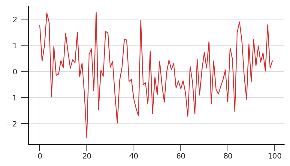
To be precise, these are the recorded values:
x = [ 1.76405235, 0.40015721, 0.97873798, 2.2408932 , 1.86755799, -0.97727788, 0.95008842, -0.15135721, -0.10321885, 0.4105985 , 0.14404357, 1.45427351, 0.76103773, 0.12167502, 0.44386323, 0.33367433, 1.49407907, -0.20515826, 0.3130677 , -0.85409574, -2.55298982, 0.6536186 , 0.8644362 , -0.74216502, 2.26975462, -1.45436567, 0.04575852, -0.18718385, 1.53277921, 1.46935877, 0.15494743, 0.37816252, -0.88778575, -1.98079647, -0.34791215, 0.15634897, 1.23029068, 1.20237985, -0.38732682, -0.30230275, -1.04855297, -1.42001794, -1.70627019, 1.9507754 , -0.50965218, -0.4380743 , -1.25279536, 0.77749036, -1.61389785, -0.21274028, -0.89546656, 0.3869025 , -0.51080514, -1.18063218, -0.02818223, 0.42833187, 0.06651722, 0.3024719 , -0.63432209, -0.36274117, -0.67246045, -0.35955316, -0.81314628, -1.7262826 , 0.17742614, -0.40178094, -1.63019835, 0.46278226, -0.90729836, 0.0519454 , 0.72909056, 0.12898291, 1.13940068, -1.23482582, 0.40234164, -0.68481009, -0.87079715, -0.57884966, -0.31155253, 0.05616534, -1.16514984, 0.90082649, 0.46566244, -1.53624369, 1.48825219, 1.89588918, 1.17877957, -0.17992484, -1.07075262, 1.05445173, -0.40317695, 1.22244507, 0.20827498, 0.97663904, 0.3563664 , 0.70657317, 0.01050002, 1.78587049, 0.12691209, 0.40198936]
Now, we need to know how many pulses are inferred if we use a detection threshold of 1 mean + 1 standard deviation. We got THREE different results based on the implementation:
- Python implementation: 9 bursts
- R implementation: 11 bursts
- Octave implementation: 12 bursts
The implications are concerning. If such a basic operation produces different results, what other disparities might exist in more complex algorithms? Are other discrepancies due to language and operating systems (I tested the method on the same laptop)? Is our assumption of cross-platform consistency fundamentally flawed?
In the next post, I’ll explore why these differences occur and discuss potential solutions. For now, remember: when porting algorithms between languages, verify every numerical operation, no matter how basic it seems.
Octave code
output_precision (10)
b = fir1(2, [0.1, 0.2], "bandpass")
% b =
%    0.06310305169   0.88754953849   0.06310305169
x_filtered = filtfilt(b, 1, x);
y = x_filtered > mean(x_filtered) + std(x_filtered);
y = [0 y 0];
intervals = [find(diff(y)>0)', find(diff(y)<0)'];
size(intervals)
% ans =
%    12    2
intervals
% intervals =
%     1    2
%     4    6
%    12   13
%    17   18
%    25   26
%    29   31
%    37   39
%    44   45
%    73   74
%    85   88
%    92   93
%    98   99
Python code
b = scipy.signal.firwin(2+1, [0.1, 0.2], pass_zero="bandpass", window="hamming", scale=1)
b
# array([0.06301614, 0.88770441, 0.06301614])
x_filtered = scipy.signal.filtfilt(b, [1], x)
y = np.array(x_filtered) > (np.mean(x_filtered) + 1*np.std(x_filtered))
y = np.concatenate([[0], y, [0]])
interval_start = np.nonzero((np.diff(y)>0))[0]
interval_stop = np.nonzero((np.diff(y)<0))[0]
intervals = np.vstack([interval_start, interval_stop]).T
intervals.shape
# (9, 2)
intervals
# array([[ 5, 7],
#        [16, 18],
#        [31, 33],
#        [46, 47],
#        [49, 50],
#        [52, 53],
#        [57, 58],
#        [74, 75],
#        [88, 89]])
R code
library(signal)
b = signal::fir1(2, c(0.1, 0.2), "pass", window="hamming")
b
#[1] 0.06310305 0.88754954 0.06310305
x_filtered = signal::filtfilt(b, x)
y = x_filtered > (mean(x_filtered) + sd(x_filtered))
y = c(0, y, 0)
intervals = cbind(which(diff(y) > 0), which(diff(y) < 0))
dim(intervals)
# [1] 11  2
intervals
#       [,1] [,2]
#  [1,]    1    2
#  [2,]    3    6
#  [3,]   12   13
#  [4,]   17   18
#  [5,]   25   26
#  [6,]   29   31
#  [7,]   37   39
#  [8,]   44   45
#  [9,]   85   88
# [10,]   92   93
# [11,]   98   99